Introducing tree “node elevation” to replace both “node depth and “node height”.

A tree’s nodes may be assigned a depth and a height. If you would like to brush up on these concepts, then baeldung.com has a great explainer article Difference Between Tree Depth and Height. The difference may be summarised as

MeasureMeasures what?
The height difference between the node and the most distant member of the zero-reference set:
node depthroot node
node heightleaf nodes
What is the differentiator between the two measures?

Notice that the definitions of depth and height differ only in which is the zero-reference level for the measurement.

The weakness of current terminology is in two aspects:

  • calling the measures ‘depth’ and ‘height’ hides the essential difference between them which is the chosen zero-reference node(s) set.
  • there are other possible zero-reference sets (example below) and for all of these other zero-reference sets some nodes will be above the zero-reference (higher or positive elevation) and some nodes will be below the zero-reference (lower or deeper).

Relationship between Height, Depth and Elevation

Elevation is a single scale that incorporates both height and depth. Height is positive, and depth is negative with respect to a zero-reference level. This is shown in the following geographic example.

Colour three-dimensional regional elevation image of the northern Gulf of Eilat/Aqaba.

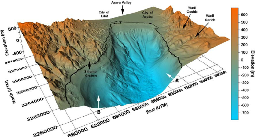
The zero reference (black line) is sea-level with the highest land at 600m and the deepest water at 700m. This corresponds to elevations between +600m (land height) and -700m (water depth).

Elevation from …

This article argues for replacing node depth and node height with the following:

Existing measureElevation from …
height (+ive)Elevation from Leaves (+ive)
depth (+ive)Elevation from Root (-ive)

The definition of elevation is exactly as currently defined for height and depth, with the exception that the sign of an elevation below the zero-reference level will be negative.

Other zero-reference levels

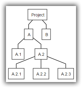
Defining elevation in this way allows us to consider other zero-reference levels in a tree. Here is a practical example taken from the domain of Project Management. The tree represents the project Work Breakdown Structure (WBS).

Project Management WBS.
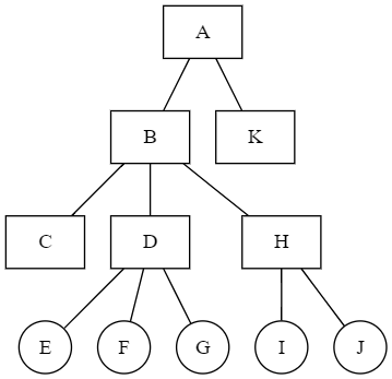
‘A’ and ‘B’ are Summary Elements. ‘C’ and ‘K’ are Planning Packages. ‘D’ and ‘H’ are Work Packages with activities associated with them. And ‘E’, ‘F’, ‘G’, ‘I’ and ‘J’ are Activities.

The set of nodes {C, D, H, and K} are the leaf nodes in the WBS and form an interesting zero-reference level for the tree. Let’s call this the “WBS Leaves” zero-reference set.

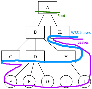
Here are the Root, Leaves, and WBS Leaves elevations for all nodes:

NodeRoot ElevationWBS Leaves ElevationLeaves Elevation
A023
B-112
C-200
D-201
E-3-10
F-3-10
G-3-10
H-201
I-3-10
J-3-10
K-100
Elevations for each node

This zero-reference level is useful in Project Management because it allows us to give precise definitions for commonly used terms:

  • The WBS consists of all nodes with a non-negative “WBS Leaves” Elevation.
  • Summary Elements may be defined as nodes with “WBS Leaves” Elevation greater than zero.
  • Work Packages may be defined as nodes with “WBS Leaves” Elevation of 0 and “Leaves” Elevation of 1.
  • Planning Packages may be defined as nodes with “WBS Leaves” Elevation of 0 and “Leaves” Elevation of 0.
  • Activities may be defined as nodes with “WBS Leaves” Elevation of -1 and “Leaves” Elevation of 0.

Applied Category Theory

Recently I reached out to Simon Willerton about applying Category Theory to Project Management models, here is the response.

Putting Project Management models on a sound footing.

Hi Simon,

Thanks for your article on the Project Management Schedule Network as a category. Category theory may have a broader role in putting project management models on a sound footing.

If we include the Work Breakdown Stucture into the model, a central issue is maintaining coherence between the Schedule Network view (as discussed in your article above) and the Work Breakdown Structure view of the same activity.

… schedule activities participate in both the WBS tree structure (“leaf” nodes under the work packages) and in the schedule network (network nodes). The schedule activities are the “atoms” from which both the WBS tree structure and the schedule network are built. This means that the WBS and schedule network are maps of the same territory, and should, therefore be coherent. However, this observation is at wide variance to the experience of many project managers. Keys for Agile Co-Evolution of the WBS and Schedule Network: The “Schedule Network 100 Percent” Rule and the “Add and Prune Dependencies” Algorithm David Pratten, PMP – February 5, 2016

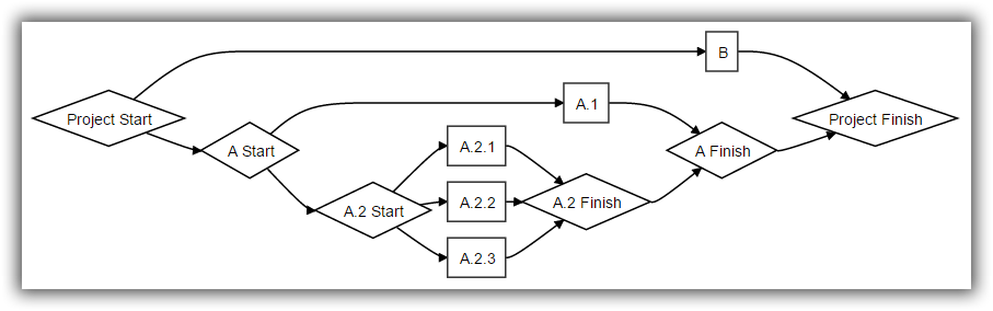
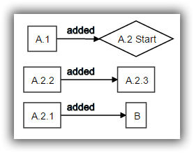
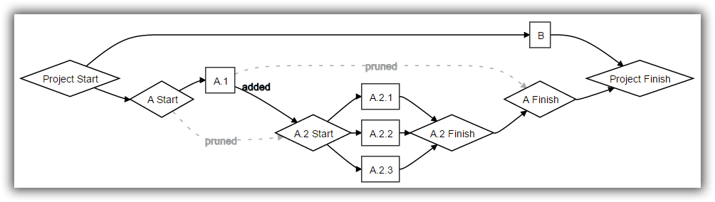
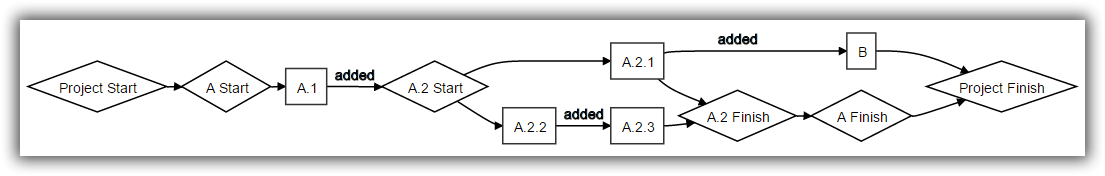
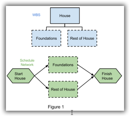
The initial step of converting the WBS to a Coherent Schedule Network looks like a functor: WBS to Coherent Schedule Network Functor

My intuition is that sequencing by adding dependencies and pruning while preserving coherence with the WBS is also a functor but I am less certain of that. Add Dependencies and preserve coherence with WBS

Ken Scrambler’s Lambda Jam 2019 – Applied Category Theory talk has inspired.

Are you aware of work going on in applying category theory to project management modelling?

David

Posted by: David Pratten on September 1, 2019 11:18 AM | Permalink | Reply to this

Re: Putting Project Management models on a sound footing.

Apologies for my rather tardy response, David. This certainly looks interesting, although I am quite ignorant of the vast majority of project management notions.

I don’t know of any work going on applying category theory to project management modelling at the moment. I know that a couple of (applied) category theorists have expressed interest in this to me, but I think they are working on various other things at the moment, as am I. My hope is to think seriously about this in a year or two when I’ve managed to get other projects off my plate.

Posted by: Simon Willerton on October 6, 2019 10:03 PM | Permalink | Reply to this

Using a Gantt Chart to Show Schedule Uncertainty

Temporary organisations (or projects) frequently work with uncertain timelines. Briefing senior management on the extent of uncertainty and progress towards reducing uncertainty is a crucial Project Management challenge. This article explores a visual approach to communicating schedule uncertainty using the common Gantt chart.  The approach taken is to show the Gantt Chart, and then explain the various elements in it.

Key Messages

The Gantt Chart is amenable for illustrating the following project talking points.

  • This project will require schedule contingency due to the parallel work involved.
  • The estimates for the series and parallel tasks are identical at 100 days.
  • Earlier activities have less schedule uncertainty,  later activities have more schedule uncertainty. This is because later activities are affected by the accumulated uncertainty of prior activities.
  • Even with uncertainty added (at +/- 20%)  the Optimistic and Pessimistic Finish  times for both series and parallel tasks are identical.
  • But in the real world, doing work in parallel means that following activities are affected differently to activities done in series.  (Illustrating merge bias.)
  • The parallel tasks are likely to be delayed from a week up to a month more than the series tasks depending on how many prior parallel tasks that are depended on.
  • This project will require significant schedule contingency due to the parallel work involved.

The project activities

  • Series Tasks
    • [Task Series 1-10] ten tasks which are in series (10 days each) .
  • Parallel Tasks
    • [Task Parallel 1-5] five tasks in parallel (50 days each)
    • [Task Depends on Parallel 1-x] five tasks (50 days each) which depend on from 1 to 5 earlier tasks in parallel.

Uncertainty

Task duration uncertainty is frequently modeled using the BETA, Triangle, and Normal random distributions. In this example the activity uncertainty has been modeled as normally distributed with a mean equal to the task’s nominal duration and a standard deviation of +/-20%.  The Optimistic/Pessimistic Duration is defined as Duration +/- 2 * Standard Deviations which spans ~95% of expected durations.

Chart Bar

Each Gantt Bar shows six events:

Events

Event How is it calculated?
Optimistic Start The Start/Finish time for the activity if every activity’s duration is the optimistic shortest time.
90% Start Based on Monte Carlo simulation, 90% of the time the task will have started by this time.
Likely Start/Finish The most likely Start/Finish Date based on a Monte Carlo simulation.
90% Finish
Based on Monte Carlo simulation, 90% of the time the task will have finished by this time.
Pessimistic  Finish The Finish time for the activity if every activity’s duration is the pessimistic longest time.

Merge Bias

The diagram nicely illustrates Merge Bias.  The last four activities all have later likely start dates.  The later times are due to the increasing numbers of prior tasks that need to complete in parallel. That is, more parallel completions equals later expected start time.

How was this created?

The Likely Start and Finish times and 90% Start and Finish times are calculated  using a 2000-run Monte Carlo simulation within MS Project. The code supports both the Triangle and Normal Distributions for capturing activity uncertainty. The input data and results of this run may be found as a CSV file Compare Series and Parallel.csv. The project start date was Sun 25-Feb-18 and scheduling was done from the Project Start Date with the Standard 5 day a week calendar. Let me know if you are interested in reviewing the code, and I will tidy it up and make it available on Github.

The visualisation was created using the following MS Project Bar Styles:

Other options

While I have been unable to find an existing example of presenting the output from a Monte Carlo run as a Gantt Chart, the idea of using the Gantt Chart to present schedule uncertainty is not original. Here are a couple of prior examples:

There are many examples available that show schedule uncertainty as a histogram of end dates.  Glen Alleman shows a good example here. Palisade have visual examples here. And a Statistical Pert example here.

Estimating – Reading

For inspiration on estimating – check out this resource list from Glen Alleman at “Herding Cats” – How to estimate anything

Lean – reading

I am convinced that Lean thinking and work patterns are crucial for IT-related change projects and the IT Service Management portfolio. When I am seeking inspiration I dive into:

Lean Production Simplified, Third Edition: A Plain-Language Guide to the World’s Most Powerful Production System B0169UYCEE (book) by Pascal Dennis. Dennis in his 3rd Ed. includes specific material on bridging from the factory floor to knowledge work. The argument that LEAN is important to knowledge work is persuasive – the challenge is in application.


The Remedy: Bringing Lean Thinking Out of the Factory to Transform the Entire Organization B003V89YW8(book) by Pascal Dennis.  Not as sharp as “Lean Simplified” but a useful guide to bridging across from production to business contexts.

Keys for Agile Co-Evolution of the WBS and Schedule Network: The ‘Schedule Network 100 Percent’ Rule and the ‘Add and Prune Dependencies’ Algorithm

projectmanagement.com Knowledge Shelf just published an article of mine on “Keys for Agile Co-Evolution of the WBS and Schedule Network: The ‘Schedule Network 100 Percent’ Rule and the ‘Add and Prune Dependencies’ Algorithm

Abstract

The ‘schedule network 100 percent’ rule and the ‘add and prune dependencies’ algorithm are keys for enabling the agile co-evolution of the work breakdown structure (WBS) and the schedule network. While creating and maintaining coherence between the WBS and schedule network has never been easy, today’s pressures to move toward a more agile practice of project management increase the challenge. This article elaborates on current, best practice project management foundations and adds the necessary definitions and methods for defining what coherence between the WBS and schedule network means and the methods to automatically create and maintain such coherence. The goal is project management practice where full coherence between the WBS and schedule network is taken for granted and maintained without effort by the project planner.

Read more …

Starting a project late is worse that finishing it late

Over the last few years of reading Glen Alleman’s “Herding Cats” blog, I have come across the refrain “Risk Management is how adults manage projects” many times.  Today, I chased down the source of this quote to Tim Lister’s 2004 “How Much Risk Is Too Much Risk?” talk. I’m glad I did. Among the many gems on risk management there, my two favourites are linked to Tim’s refreshing focus on value, and the accountability of the client.  The first key idea is:

Starting a project late is worse that finishing it late

and the second:

The only reason to quantify cost (schedule and budget) is to have something to compare to your quantification of benefit.

which doesn’t make too much sense without Tim’s explanation.  If you are curious, effort to dig up this talk and read it will be rewarded.

Alternatively, check out Tim’s talk at InfoQ London 2014 “Risk Management is Project Management for Grown-Ups” which contains this thought of the day

All the projects with benefits but no risk were completed a long time ago.

Risk and Safety discussion

Having identified our risks we then proceed to characterise the source, the causal mechanisms, the consequences, identify controls and finally apply some sort of ranking to the risk. Sounds fairly straightforward and objective doesn’t it…

and

Although dangers are real, there is no such thing as objective risk or real risk. Even the simplest, most straightforward risk assessments are based on theoretical models, whose structure is subjective and assumption laden and whose inputs are dependent on judgement

From Matthew Squair’s excellent “System Safety” lecture slides.

PMQu: A Quality Tool for Project Information in MS Project

pmicriticalpath201504(Article published first in “The Critical Path”, PMI Sydney, April 2015)

The open source add-in for MS Project called œPMQu assists project managers to create, and maintain, quality-checked project information. Earlier in this series of articles, I argued[1] for greater coherence between the WBS and Schedule Network, and then in the second article [2] introduced the means to automate this coherence by applying the new Schedule Network 100 percent rule and the Add and Prune Dependencies algorithm. This article introduces PMQu, a MS Project add-in that implements this rule and algorithm and other best practice quality checks. Firstly, we review the benefits of quality checking project information, and then, after pointing to the sources of the quality checks, the PMQu add-in is introduced and the article concludes with a short invitation to explore next steps.

Context, and why perform quality checks?

Managing quality, including that of project plans, is a management challenge involving both people and process. PMQu will automate just one aspect of process, which is, checking the conformance of plans to pre-agreed quality standards. This is an activity which is impractical to perform manually on real-world plans.

PMQu is intended for the professional project manager and Project Management Office (PMO) where each project’s WBS and Schedule Network may be contained within a single stand-alone MS Project plan of up to 300-350 activities. In this context there are at least four reasons for checking the quality of project information. Quality checking can:

  • Reduce, or eliminate, many common WBS and Schedule Network mistakes,
  • Improve the flexibility of schedules under rolling wave planning,
  • Improve the transferability of project plans between project managers,
  • Assist managers to induct new project managers to use a common style for project information.

For this context, from where has the author drawn the quality checks?

Sources of Quality Checks

Firstly, PMQu checks the coherence between the WBS and Schedule Network using the Schedule Network 100 percent rule and the Add and Prune Dependencies algorithm that were referred to earlier.

Secondly, and equally importantly, PMQu performs quality checks according to best practice guidance found in the following six recommended sources:

Naturally, not every piece of advice is checked.  Instead, PMQu checks an integrated set of guidance drawn from all these sources.

PMQu Add-in for MS Project

The PMQu open source add-in for MS Project 2010/2013 reads the current project and creates a report in the user’s browser covering 42 separate checks.  PMQu does not alter the current project.  Table 1. contains a breakdown of the quality checks by area with some examples:

Quality Check Area # of Checks Example Checks
Task Identity 4 Every task must have a unique name.
Work Breakdown Structure 7 Every summary component will have a minimum of two child components.The WBS will be coherent with the Schedule Network.
Schedule Network 12 Summary Tasks may not have dependencies.All tasks will participate in the Schedule Network.
Resources 4 Summary Tasks may not have resources assigned.
Scheduling 10 All tasks must have a duration specified.
Progress 5 Milestone’s %Complete must either be 0% or 100%.
Microsoft Project settings 18 Schedule From [Project Start Date].
TOTAL 42  

Table 1. “ A breakdown of the quality checks with some examples

Next steps

You are invited to install, and use, PMQu under the open source MIT license. The software itself, a list of all the checks, sample plans, and the installation and usage instructions may be found on GitHub at https://github.com/DavidPratten/PMQu . Your comments and questions are welcome via GitHub issues.

The author relies on the PMQu add-in for MS Project to check project information quality for his projects. How will you use it? The MIT license for the software means that you are free to use the intellectual property in this software for anything, including running your projects, as a resource for your PMO, for training project managers, and creating commercial opportunities. Go for it!

[1] Pratten, D. (2014). Having a common definition of œdeliverable in both WBS and the schedule network The Critical Path, 5(6), 16-17.  Retrieved from http://www.pmisydney.org/index.php/document-repository/doc_download/908-critical-path-december-2014

[2] Pratten, D. (2015). WBS and Schedule Network coherence at scale The Critical Path, 6(1), 14-16.  Retrieved from http://www.pmisydney.org/index.php/document-repository/doc_download/986-criticalpath201502volume6issue1

WBS and Schedule Network coherence at scale

pmisydcp022015(Article published first in “The Critical Path”, PMI Sydney, February 2015)

As argued in a previous article[1], common definitions of œdeliverable in the WBS and schedule network may be maintained by having œStart and œFinish milestones in the schedule network for each WBS summary component. This article introduces a œSchedule Network 100 percent Rule and the œAdd and Prune Dependencies Algorithm by which we can automate this coherence between the WBS and schedule network at project scale. The Schedule Network 100 percent Rule is applied to a WBS to derive an initial schedule network. Required dependencies are then added to the initial schedule network and redundant dependencies are pruned, using the newly introduced œAdd and prune dependencies algorithm. The result is a sequenced schedule network that is coherent with the WBS. A following article will introduce open source software that implements this algorithm and supports the progressive elaboration of a project plan under rolling wave planning.

The 100 percent rule

The Schedule Network 100 percent Rule allows us to construct an initial, fully connected, schedule network based solely on the WBS. The well-known WBS 100 percent rule states[2]: œThe next level decomposition of a WBS element (child level) must represent 100 percent of the work applicable to the next higher (parent) element. Both the WBS and the schedule network are œmaps of the same territory and use different visual languages to represent the deliverables of the project. This article introduces[3] the Schedule Network 100 percent Rule which may be stated as: œA summary activity’s start milestone must precede, and its finish milestone must succeed, 100 percent of the work applicable to the summary activity.

100rule-23

Diagram 1. Sample WBS

Let’s apply the Schedule Network 100 percent Rule to the sample WBS in Diagram 1.

We create a schedule network with œStart Project and œFinish Project milestones before, and after, 100 percent of the project’s work. We place Start and Finish milestones before, and after, 100 percent of A’s work, and before and after A.2’s work. The result is a fully connected, but unsequenced, schedule network (Diagram 2.) that is coherent with the WBS


100rule-24

Diagram 2. “ WBS Coherent Schedule Network

Schedule Network 100% Rule animation

Click on the play button for a step-by-step animation of and example application of the Schedule Network 100% Rule.

Add and Prune Dependencies

The new[4] Add and Prune Dependencies Algorithm allows us to automatically construct a fully sequenced and simplified schedule network coherent with the WBS.

Often, activities and planning packages are sequenced and then open ends are joined to form a completed schedule network, however, when we do this, coherence with the WBS is not preserved. Instead, we start with a fully connected, but unsequenced schedule network (Diagram 2. above) and use the œAdd and Prune Dependencies algorithm to sequence the activities and simplify the plan while ensuring that the Schedule Network 100 percent Rule is maintained.

The Add and Prune Dependencies algorithm has two phases:

  1. Add a dependency, and then
  2. Simplify by pruning any other dependencies that are now redundant and are no longer required by the Schedule Network 100 percent Rule.

In our example the schedule network needs to be sequenced with the following dependencies (Diagram 3.).

Diagram 3. Dependencies to be added.

Diagram 3. Dependencies to be added.

Adding the first dependency (A.1 to A.2 Start) and applying the Add and Prune Dependencies Algorithm gives us the Schedule network shown in Diagram 4. It shows the added dependency as well as the dependencies that have become redundant and marked for pruning. The two dependencies may be pruned because they are no longer necessary for maintaining the Schedule Network’s 100 percent Rule. The dependency from œA Start to œA.2 Start may be pruned because the newly added dependency ensures that œA Start precedes œA.2 Start.  Similarly, the dependency from œA.1 to œA Finish may be pruned because the newly added dependency ensures that œA Finish succeeds œA.1.

Diagram 4. Adding the first dependency.

Diagram 4. Adding the first dependency.

After adding the remaining two dependencies (from A.2.1 to A.2.2 and from A.2.1 to B) and automatically pruning three redundant dependencies, we get a fully sequenced schedule network (Diagram 5.) that continues to satisfy the Schedule Network 100% Rule and is therefore coherent with the WBS. Critical path and other scheduling algorithms may now be run on the completed network.

Diagram 5. The sequenced, simplified and WBS-coherent schedule network.

Diagram 5. The sequenced, simplified and WBS-coherent schedule network.


Add and Prune Dependencies Algorithm animation

Click on the play button for a step-by-step animation of the Add and Prune Dependencies Algorithm.

Add and Prune Dependencies Algorithm animation

This article has introduced a new Schedule Network 100% Rule and the Add and Prune Dependencies Algorithm and show how they, together, allow us to derive a schedule network that incorporates required dependencies and is both 1) as simple as possible, and 2) fully consistent with the WBS. This ensures that the WBS and schedule network share a common vocabulary of œdeliverables and automatically ensures that the schedule network avoids open ends. A following article will introduce open source add-in to MS Project that implements this rule and algorithm.

[1] Pratten, D. (2014). Having a common definition of œdeliverable in both WBS and the schedule network The Critical Path, 3(6), 16-17.

[2] Haugan, Gregory T. (2002). Effective Work Breakdown Structures. Vienna, VA Management Concepts.

[3] No prior descriptions of the Add and Prune Dependencies Algorithm were found in the existing Project Management literature.

[4] No prior descriptions of the Schedule Network 100 percent Rule were found in the existing Project Management literature.

Having a common definition of œdeliverable in both WBS and the schedule network.

(Article published first in “The Critical Path”, PMI Sydney, December 2014)

Having a common definition of œdeliverable in both WBS and the schedule network assists project managers to build a common understanding of the project scope and progress amongst stakeholders. This article examines possible causes for the divergence of the schedule network’s definitions and those of the WBS and argues that it is best practice to follow the example of Figure 6-21 in the PMBOK(r) Guide 5th Ed. and include a œStart and œFinish milestone in the schedule network for each WBS component. At project scale, implementing this practice requires automation help and a following article will explain a new project management algorithm œAdd and Prune Dependencies which enables this.

The project model has, at its heart, the dual structures of the tree-like Work Breakdown Structure (WBS) and the schedule network. Both the WBS and the project schedule are œmaps of the same territory and use different visual languages to represent the deliverables of the project. In the WBS the top-level component represents 100% of the deliverables or products of the project, and each level below decomposes the same 100% into smaller components that represent part of the deliverables. In the schedule network 100% of the deliverables of the project are represented between the œStart Project and œFinish Project milestones. Likewise, smaller deliverables may be represented by pairs of milestones that mark the start and completion of these deliverables.

Outside of domains that rigorously apply Earned Value Management (EVM), it is common for the deliverables defined in the WBS to not be precisely traceable to milestones in the schedule network. Assuming that dependencies are not placed on, so called, œSummary tasks, the planner will commonly create œDeliverable completed milestones in the schedule network to represent the availability of interim deliverables and the point where work that depends on those interim deliverables can begin. However, manually created œDeliverable completed milestones are likely (and with updating over time, inevitable) to not exactly correspond to the completion of any WBS component. There are two main reasons for this. Firstly, the selection of predecessor relationships for the œDeliverable completed milestone is unlikely to correspond exactly with the set of predecessors required to match the completion of a WBS component, and secondly, the choice of deliverables highlighted by œDeliverable completed milestones may be dominated by tactical considerations at a detail planning level rather than the set of deliverables already defined in the WBS. As the project progresses, this can result in a widening mismatch between the WBS œmap and the schedule network œmap.

So how can a WBS and schedule network be provably based on the same set of deliverables?

Critical Path Article 01.01

Figure 1 shows the simplest case of a two level WBS with two planning packages at the lowest level and its corresponding schedule network prior to sequencing. Notice that the œHouse deliverable is represented in the schedule network by two milestones œStart House and œFinish House. In general this is true. The implication is that if we want to have common definitions of œdeliverable in both the WBS and schedule network, each component in the WBS will be mirrored by œStart and œFinish milestones in the schedule network.

The thesis of this article is that definitions of deliverables will inevitably diverge if the schedule does not maintain œStart and œFinish milestones matching each WBS component, and that their presence in the schedule will create the alignment of definitions that we are looking for. Interestingly, while PMI’s best practice guidance is largely silent on this question, Figure 6-21 on p183 the PMBOK(r) Guide 5th Ed. shows an example of exactly this with œStart and œFinish milestones in the schedule network that correspond to WBS components.

Outside of domains that rigorously apply EVM this is not (yet) common practice, but aligning the WBS and the schedule network’s deliverable definitions means that the readers of the WBS and the readers of the schedule network are speaking the same language and that progress information can be trivially mapped back to the completion of WBS components. At project scale this requires automation support and the next article will describe the new œAdd and prune dependencies algorithm which facilitates this.

“Ready for use” and “Ready to use”

I am prompted to write because of a useful paper: “Perspectives on the Formal Authority Between Project Managers and Change Managers”  in the October/November 2014 Project Management Journal by Julien Pollack and Chivonne Algeo both of the University of Technology, Sydney.

I am in broad agreement with the authors on:

… project management focusing on … issues, including scheduling, managing a budget, change control, and procurement, whereas change management focuses on … activities, such as empowering change agents, developing a senior guiding coalition, ensuring their support, and removing organizational obstacles.

however I would have expressed it a bit differently.

For a project to deliver business value, broadly speaking, two things need to show up simultaneously at a future date:

  1. the technical deliverable (building, IT system, transport system,…) needs to be ready for use by the people, and
  2. the people need to be ready to use the technical deliverable.

The trick is that the disciplines that are involved in each like chalk and cheese.  As project scale increases it becomes difficult for one human mind to stay with both disciplines.  It is about as easy as simultaneously enjoying fine classical music in one ear and fine jazz in the other. So while one person (e.g. let it be a Project Manager) may be responsible for both the technical deliverable and the people side of change, in practice the two sides of the project are “uneasy bedfellows”. As the authors note earlier in the paper, the

These differences suggest that project managers and change managers do not see their managerial roles in equivalent ways.

The implications suggested by the authors for the relationship between project managers and change managers are compelling:

For project managers, the implications of this research suggest a need to find some balance between the need for control and direction that comes with a single point of account ability, and allowing change managers to have a distinct area of responsibility that they can deliver in their own way, while maintaining coordination between the project management and change management aspects of organizational change projects.


Foundations of Project Management

This is a collection of references to articles and ideas that I refer to constantly to refresh my vision for Project Management.

Bent Flyvbjerg on Reference Class Forecasting.

Mel Conway on How committees Invent. The collaboration patterns of project stakeholders determines more than might be expected.

Fernando Flores on Conversations for Action. This is the project Manager’s daily bread. See my reflection on this:  What Could Possibly go Wrong.  See Crockford and Marshall’s application of this to Project Management. See also Peter Dennings excellent article ((Peter J. Denning. 2013. The other side of language. Commun. ACM 56, 9 (September 2013), 35-37. DOI=10.1145/2500132 http://doi.acm.org/10.1145/2500132)) .

Atul Gawande on 1846683149  The Checklist Manifesto: How to Get Things Right. Atul Gawande. How do we ensure repeatable processes with highly qualified professionals? How can we document them?

0814417817Tom Kendrick on Results Without Authority: Controlling a Project When the Team Doesn’t Report to You. The project manager’s toolkit as sources of power for good.


Patterson, Grenny, McMillan, and Switzler on Crucial Conversations.  Required reading only if the project manager per chance encounters situations where options vary, the stakes are high and emotions run strong.

Expected % Complete MS Project Custom Column

I attended Angela Chellas’ MS Project Advanced workshop today (excellent course) and there was a question about how to figure out what % complete that a task should be if it was on track.  Based on elapsed time, the Expected % Complete for tasks and summary items may be calculated using a MS Project Custom Field.

[expand title=”Text of the formula – to paste in.”]

Int(
  IIf([Current Date]>=[Start]
     ,IIf([Current Date]<=[Finish],
        IIf([Duration]>0,
           ProjDateDiff([Start],[Current Date])/[Duration]*100
           ,IIf([Current Date]>=[Start],100,0))
        ,100)
     ,0)
)

[/expand]


You create the custom column like this.

customcol2

PRINCE2 Joined-Up

The core of PRINCE2 project governance guidance is summarised in the introduction to the business case …

The ongoing and ever-present decision regarding the Business Case is whether the project can (still) be justified. This is based on whether the project is desirable (the cost/benefit/risk balance), viable (the project can deliver the products) and achievable (the products can provide the benefits).

The Senior User(s) is responsible for specifying the benefits and subsequently realizing the benefits through the use of the products provided by the project. The Executive is responsible for ensuring that those benefits specified by the Senior User(s) represent value for money, are aligned to corporate objectives, and are capable of being realized. ((OGC (Office of Government Commerce) (2009). Managing Successful Projects with PRINCE2 (2009 ed.). TSO (The Stationery Office).))


The following diagram captures the key PRINCE2 roles, and their concerns.  I have found this diagram very useful when socialising the PRINCE2 project patterns with project stakeholders.

PRINCE2 Joined-Up


Talking Points

  • Project is a temporary organisation to turn the inputs into the benefits.
  • Project Objectives (start with the end in mind)
    • Benefits
    • Scope and Quality of Products
    • Time, Cost, and Risk appetite Inputs
  • Executive Role1
    • Key concern: Desirable8? If we had the time, cost and risk appetite would we purchase these benefits?
    • The details of the project product are not in focus.
  • Benefits2
    • Benefits are in business terms (customer impact, costs (e.g. head count), income (e.g. new capabilities and services)
  • Senior Users3
    • Key concern: Achievable4? If we receive the promised products to the required scope and quality, can we use them in the business to deliver the benefits?
  • Products5
    • What is required to achieve the benefits? The product is often an artifact (e.g. consumer product, IT system, building facility)  of some kind combined with people ready to use it.
  • Senior Suppliers6
    • Key concern: Viable7? If we were given the time, budget, and risk appetite, can we deliver to the required scope and quality?
  • Input
    • Time, Budget, People, Risk appetite