N-place implicational tautologies

Diving into Mathematical Logic brought me across Peirce’s Law, which uses the logical implication ⇒ operator only and is always True irrespective of what its two inputs (say) P and Q are:

((P ⇒ Q) ⇒ P) ⇒ P

Tower of N-place implicational tautologies

This got me thinking about the possibility of logical formulae that only use the logical implication ⇒ operator and are always True for any number of inputs.

A Hierarchy of Laws

I investigated this with some Python code and it turns out that there is a hierarchy of Laws:

Number of Variables – ArityVariablesNumber of Shortest TautologiesShortest Tautologies
(Unique up to variable renaming)
Comments
01True
1P1P ⇒ P
2P, Q2P ⇒ (Q ⇒ P)
P ⇒ (Q ⇒ Q)
Peirce’s Law is just one of sixteen two-variable tautologies with three ⇒ operators:
P ⇒ ((P ⇒ Q) ⇒ P)
P ⇒ (P ⇒ (Q ⇒ P))
(P ⇒ Q) ⇒ (P ⇒ Q)
P ⇒ (Q ⇒ (P ⇒ Q))
(P ⇒ Q) ⇒ (Q ⇒ Q)
P ⇒ (Q ⇒ (Q ⇒ Q))
((P ⇒ Q) ⇒ P) ⇒ P
P ⇒ ((Q ⇒ P) ⇒ P)
(P ⇒ Q) ⇒ (P ⇒ P)
P ⇒ (Q ⇒ (P ⇒ P))
P ⇒ ((Q ⇒ Q) ⇒ P)
P ⇒ (Q ⇒ (Q ⇒ P))
((P ⇒ P) ⇒ Q) ⇒ Q
P ⇒ ((P ⇒ Q) ⇒ Q)
(P ⇒ P) ⇒ (Q ⇒ Q)
P ⇒ (P ⇒ (Q ⇒ Q))
3P, Q, R5(P ⇒ Q) ⇒ (R ⇒ R)
P ⇒ (Q ⇒ (R ⇒ R))
P ⇒ (Q ⇒ (R ⇒ Q))
P ⇒ ((Q ⇒ R) ⇒ P)
P ⇒ (Q ⇒ (R ⇒ P))
4P, Q, R, S16P ⇒ (((Q ⇒ R) ⇒ S) ⇒ P)
P ⇒ ((Q ⇒ (R ⇒ S)) ⇒ P)
P ⇒ (Q ⇒ ((R ⇒ S) ⇒ P))
P ⇒ ((Q ⇒ R) ⇒ (S ⇒ P))
P ⇒ (Q ⇒ (R ⇒ (S ⇒ P)))
((P ⇒ Q) ⇒ R) ⇒ (S ⇒ S)
(P ⇒ (Q ⇒ R)) ⇒ (S ⇒ S)
P ⇒ ((Q ⇒ R) ⇒ (S ⇒ S))
(P ⇒ Q) ⇒ (R ⇒ (S ⇒ S))
P ⇒ (Q ⇒ (R ⇒ (S ⇒ S)))
(P ⇒ Q) ⇒ (R ⇒ (S ⇒ R))
P ⇒ (Q ⇒ (R ⇒ (S ⇒ R)))
P ⇒ (Q ⇒ ((R ⇒ S) ⇒ Q))
P ⇒ (Q ⇒ (R ⇒ (S ⇒ Q)))
5P, Q, R, S , T42
6P, Q, R, S, T, U132
Table of shortest tautological laws using implication alone, of increasing arity.

Reader’s feedback is welcome!

Don’t Repeat Yourself when Computing Relations

To say that I am "gobsmacked" is an understatement! The s(CASP) language fulfills a 40-year-old dream for a computer language that adheres to the "Don’t repeat yourself" philosophy.

s(CASP) was described in 2003 by Joaquin Arias, Manuel Carro, Elmer Salazar, Kyle Marple, and Andgopal Gupta. Constraint Answer Set Programming without Grounding. Here is a recent tutorial published for the language A Short Tutorial on s(CASP), a Goal-directed Execution of Constraint Answer Set Programs. And has been recently implemented in both Caio and SWI-PROLOG. And here is a recent review article s(CASP) + SWI-Prolog = 🔥.


Write your first s(CASP) program using the s(CASP) profile at https://swish.swi-prolog.org.


In this article I’ll describe by way of example, the kind of language that I have been looking for and show a small aspect of what s(CASP) can do that other languages can’t.

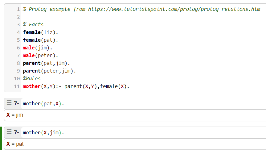
Forty years ago, in my undergraduate days, I was introduced to the logic programming language "Prolog". The premise of the language is that a Prolog program captures facts and rules and that Prolog ‘figures out’ how to order the computations required to answer a query. This Prolog Family Relationships example shows how Prolog doesn’t have a preferred direction of computation. The arguments are symmetric with regards to what is known and what is unknown.

As shown above, if we provide one argument Prolog will compute the other, or if we provide the "other", Prolog will compute the "one".

Dream Computer Language

My dream computer language has, at least, the following capabilities:

  • Capture data and computable relationships between data independent of the questions (or queries) that the programmer is currently aware of (unlike procedural languages but like DBMSs do for data)
  • Enter information once. For both data and computable relationships and allow any missing data to be computed. Another way of expressing this is that the language handles known and unknown arguments symmetrically, is indifferent to which arguments are known and which are unknown, creating a computation to find the missing arguments (as Prolog does for the computed relationship mother() and as SQL does for data)

Problem

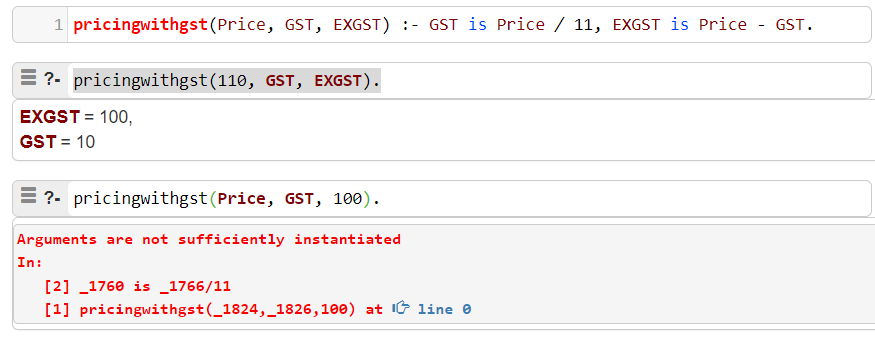
I soon discovered that Prolog doesn’t keep up its indifference to the direction of computation for long. As soon as mathematical calculations are added to Prolog the paradigm of order-independent facts and rules stops working. Consider the GST in Prolog example Prolog program to calculate a 10% GST (or VAT).

As you can see from the above example, the Prolog language will only find a solution for one direction of computation. While the definition contains enough information to compute both directions to, and from Price, Prolog is unable to do so.

How does s(CASP) compare?

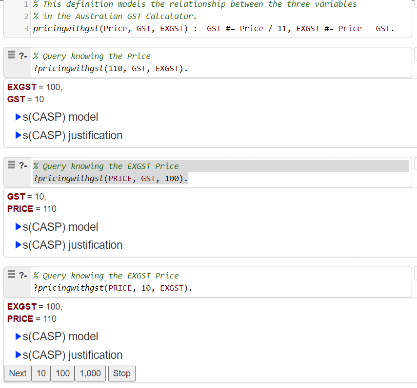
s(CASP) captures the pricingwithgst rule in a similar way to Prolog, but has a ‘super power’ it treats all the arguments to the rule symmetrically and therefore handles the GST example perfectly!

The s(CASP) program contains exactly the same information in the Prolog program and shows the symmetry of handling arguments that I have dreamed of!

Application

A programming language that allows the capturing of a computed relationship (GST being a trivial example) and then doesn’t care which arguments to the relationship are known and which are unknown can reduce the cost of building and maintaining digital models to be used for various purposes.

Following on from the GST example, it is almost certain that the code behind Australia’s GST Calculator web app contains two copies of the computed relationship between Price, GST, and Price exGST, one for each direction of calculation. If s(CASP) was behind the app then the computed relationship would be entered just once as a rule, and the two directions of computation would just be two different queries with different knowns and unknowns. s(CASP) would sequence a computation to find the missing values.

Functional Programming with SQL Query lambdas, functions and pipelines

Your input and feedback on this article are welcome on github.com/DavidPratten/sql-fp

This article aims to add lambdas, functions and pipelines to the functional programming core of standard SQL, and thereby:

  • separate transformation from data,
  • increase SQL use cases
  • increase SQL code re-use
  • reduce situations where programmers need to cross the "impedance barrier" from queries to use the procedural CREATE FUNCTION, and
  • increase processing speed through full utilisation of the query planner/ optimiser,

using an approach that may be implemented at scale with reasonable cost.

The outline of this article is as follows:

  • Introduce query lambdas and the GIVEN clause, including recursive query lambdas
  • Describe query functions and query pipelines
  • Conclude with a discussion of the benefits and costs of the proposed features.

Query Lambdas

Query lambdas are the foundation of this proposal, so we will consider them first. Query lambdas have a function signature of (table_or_sub-query, ...) -> table, that is:

  • accepting one, or more, tables or sub-queries as input
  • and returning a table.

All table references within the lambda are local to it and tables in the global namespace are invisible.

Realising Query Lambdas in SQL with GIVEN

SQL’s SELECT may be turned into a lambda by prefixing it with the proposed GIVEN clause and wrapping the whole expression in brackets. The local_tables identified in the GIVEN clause are the only ones able to be referenced in the context of the SELECT and it’s sub-queries.

Here is an example lambda that sums the supplied state level population data at the country level.

select *
FROM (GIVEN(mapping(summary_id, id), rawdata(id, amount)) 
      SELECT mapping.summary_id, sum(rawdatea.amount) amount
          FROM rawdata rawdata
              JOIN mapping mapping ON rawdata.id = mapping.id
          GROUP BY mapping.summary_id
     )((SELECT country_id summary_id, state_id id FROM states),
       (SELECT state_id id, population amount FROM population_by_states)
      );

which may be read as:

  • apply the input relation(s)
    • (select country_id summary_id, state_id id from states) which maps states to countries as the mapping table and
    • (select state_id id, population amount from population_by_states) as the rawdata table
  • and return a population summary by country.

The query inside the lambda may be reused in any context, by passing in different tables as parameters.

This particular query lambda can be transpiled to SQL-99 as:

select *
FROM (SELECT mapping.summary_id, sum(rawdatea.amount) amount
      FROM (select state_id id, population amount from population_by_states) rawdata
               JOIN (select country_id summary_id, state_id id from states) mapping ON rawdata.id = mapping.id
      GROUP BY mapping.summary_id
     );

Recursive Query Lambdas

SQL provides a recursive (iterative and fixed-point) relational transformation via the CTE. This makes SQL Turing Complete.

A GIVEN clause may be used in conjunction with the WITH clause and turns a CTE into a (potentially recursive) query lambda.

The following recursive query lambda will generate a table of the first 50 integers counting from 1.

SELECT * FROM
(GIVEN(count(n))
 WITH 
     enumerate
        AS (
            SELECT 1 AS n 
            
            UNION ALL
            
            SELECT n + 1 FROM enumerate WHERE n < (SELECT n from count LIMIT 1) 
            )
SELECT n from enumerate)((SELECT 50 n));

This query lambda transpiles to SQL-99 as follows:

SELECT * FROM
(WITH enumerate
        AS (
            SELECT 1 AS n 
            
            UNION ALL
            
            SELECT n + 1 FROM enumerate WHERE n < (SELECT n from (SELECT 50 n) LIMIT 1) 
            )
SELECT n from enumerate);

Let’s now look at how query lambdas are the building blocks for query functions and pipelines.

Query Functions

SQL provides the VIEW mechanism to name queries, and the GIVEN clause causes VIEWs to become parameterised. Our example query lambdas may be turned into query functions summarise() and generate_series() as follows:

CREATE VIEW summarise(summary_id, amount) AS
    GIVEN (mapping(summary_id, id), rawdata(id, amount))
    SELECT mapping.summary_id, sum(rawdatea.amount) amount
    FROM rawdata rawdata
             JOIN mapping mapping ON rawdata.id = mapping.id
    GROUP BY mapping.summary_id;
)

and

CREATE VIEW generate_series(n) AS
    GIVEN(count(n))
    WITH enumerate
    AS (
      SELECT 1 AS n
      UNION ALL
      SELECT n + 1 FROM enumerate WHERE n < (SELECT n from count LIMIT 1)
    )
    SELECT n from enumerate;

The query function signature, or contract, is immediately visible in the first two lines of each!

The examples above include the declaration of the return table’s columns in brackets after the query function name. This is a feature of CTE’s backported to CREATE VIEW. In SQL-99 VIEWs must infer the returned columns from the provided SELECT.

Query Function Invocation

Just like regular VIEWs (and CTEs), query functions stand in a SELECT query in the place of a table. Query functions are invoked with the view_name followed by bracketed table, or subquery, parameters. Here is how we can invoke the query function summarise defined above.

SELECT *
from summarise((SELECT country_id summary_id, state_id id FROM states),
               (SELECT state_id id, population amount FROM population_by_states)
              );

And we can generate a table of 5 numbers starting with 1 with:

SELECT *
from generate_series((select 5 n));

Query Pipelines

Some data transformations may be usefully modelled as a staged pipeline of changes with each stage consuming the results of an earlier stage. Here is a simple pipeline diagram that illustrates our summarisation example modelled as a two stage transformation:

Building on the definitions of query functions and lambdas, a PIPES TO compound operator is proposed to allow functional programmers to express computations using a pipeline model.

Here is the PIPES TO operator used to express this two stage pipeline:

SELECT *
from ( (SELECT country_id summary_id, state_id id FROM states)
      PIPES TO
      summarise((SELECT state_id id, population amount FROM population_by_states) );

Notice that this invocation of summarise() has just one parameter. In this case the first parameter is provided by the PIPES TO compound operator.

Transpilation to SQL-99 is straight forward. The PIPES TO compound operator may be reduced to application of query functions, by moving the left-handed expression to be the first parameter of the right-hand expression, and thence to SQL-99 as shown above. Here is the PIPES TO reduced to query functions.

select *
from (SELECT *
      from summarise((SELECT country_id summary_id, state_id id FROM states),
                     (SELECT state_id id, population amount FROM population_by_states)
          )
     );

Discussion of costs and benefits

Adding a new feature to the SQL standard needs to have compelling benefits and manageable implementation costs.

Implementation costs

My high-level estimate is that the implementation costs are of O(costs of adding CTEs as part of SQL99). At this early stage in the lifecycle of query lambdas, functions, and pipelines there is much uncertainty, however here are a few factors that suggest that the implementation costs are manageable:

  • "Not the first rodeo" – the GIVEN clause operates similarly to the WITH clause in that it shapes the visible tables in the following SELECT
  • Equivalent to SQL-99 as demonstrated above, query lambdas, functions, and pipelines (just like VIEWs) are close to zero-cost abstractions. They may all be trivially reduced back to SQL-99 and made available to the query planner / optimiser to execute.
  • Clean introduction of new capabilities no changes to any legacy code is required,
  • Ergonomics overloading VIEWs with parameters is a natural extension and leverages user’s experience with built-in and CREATE FUNCTION functions.

Benefits

The benefits claimed for query lambdas, functions and pipelines are not novel. They are all consequences of bringing well understood functional programming patterns to the world of SQL queries. Here is a short sketch justifying the claimed benefits:

Separate transformation from data,

From the point of view of the development team, maintaining multiple hand-coded transformation queries is hard to justify. In SQL-99 the available mechanisms for abstracting transformations and reusing them (VIEWs and CTEs) work to the extent that at every invocation they are referring to exactly the same tables and columns. In SQL-99 every query is, at it’s base, hard coded to a global namespace of tables and columns. This means that there is no mechanism to cleanly separate the query transformation from the actual data that is being processed. Query lambdas, functions and pipelines provide precisely this capability for SQL.

Increase SQL use cases

By separating the data from transformations, SQL queries becomes more attractive to organisations to encode re-usable business rules which need to be applied to multiple data sets in multiple contexts.

Increase SQL code re-use

From the point of view of the broader SQL community, hand coding every solution means that there are no libraries of SQL transformations that can become a shared resource and built on. Query functions enable SQL query transformations to be defined once and used in a myriad of contexts. A good use case here would be providing a library of hierarchy handling query functions (ie recursive CTEs) which embody the graph theoretic algorithms which can be applied to any data.

Reduce situations where programmers need to cross the "impedance barrier" from pure functional code to use the procedural CREATE FUNCTION

For the developer, the necessity in SQL-99 to hand-code every transformation for each use-case motivates programmers to cross the impedance barrier to alternative technologies to reduce or eliminate code duplication. In addition, if a programmer wants to build or use a pre-packed solution then a procedural CREATE FUNCTION is the only currently available option.

Query lambdas, functions and pipelines lessen, or remove, these drivers for programmers.

Increase processing speed through full utilisation of the query planner/ optimiser,

The relational query planner/optimiser plays a crucial role in the functional nature of SQL. It is this part of the execution environment that enables:

  • queries to be reordered and elided,
  • materialised, indexed,
  • lazily evaluated and/or
  • parallelised.

In many cases the procedural code is not able to be optimised by the planner, leading to relatively poor performance.

The "Impedance barrier" between SQL queries and procedural code is not just a cognitive load for programmers, it is also a performance blockage on real world workloads. There is current research ongoing on how to convert procedural code back into CTEs so as to boost application performance.

Query lambdas, functions and pipelines enable programmers to stay within the purely function world of SQL queries which can be executed in an optimal way by the planner / optimiser.

Last word

In summary the proposed GIVEN clause develops the pure functional core of the SQL query, improves programmer ergonomics, and broadens the use-cases for SQL and promises improved application performance.

Composable Recursive Relational Queries

Your input and feedback on this article are welcome on github.com/DavidPratten/sql-fp

Hierarchical and graph data may be transformed with relational queries that are recursive, iterative, and fixed-point. These are available in SQL through the recursive Common Table Expression (CTE):

WITH RECURSIVE ...

This article argues that SQL’s CTE machinery is a distraction from the core idea of a recursive query and a hinderance to composition of queries. We propose a simpler SQL form which is equally declarative, expressive and composes nicely:

SELECT ... UNION SELECT ... FROM UNION

In addition, we explore how this form may be translated into Morel, a descendent of ML with relational queries.

Let’s begin by introducing a motivating example

Transitive Closure of a Tree

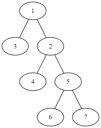
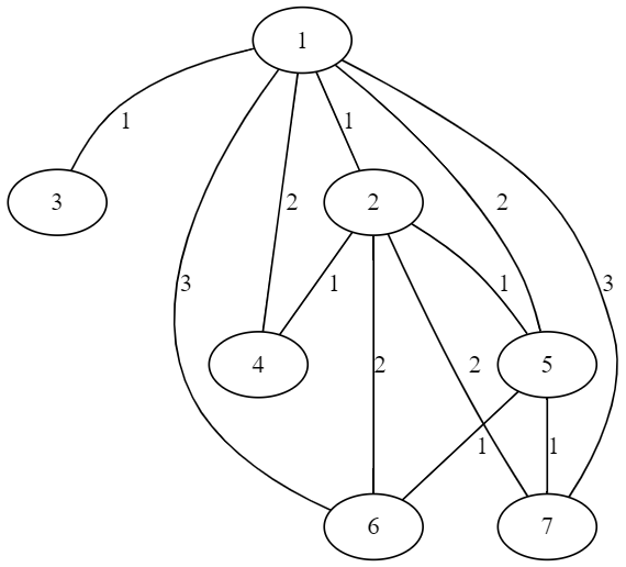
If we have a tree

Example Tree

This can be represented in a relation as:

idparent_id
11
21
31
42
52
65
75

The transitive closure of the tree is:

Transitive Closure of the Tree with depth shown on the edges

And this may be represented by the following relation.

idparent_idlevel
110
220
330
440
550
660
770
211
311
421
521
651
751
412
512
622
722
613
713

Recursive CTE query

Using the Sqlite CTE form here is the query that computes the Transitive Closure given the Tree.

/* WITH RECURSIVE transitive closure of a tree (SQLITE)
   n.b. Tree's root node convention is id = parent_id
*/
with items (id, parent_id) as (
    select 1 id, 1 parent_id
    union
    select 2, 1
    union
    select 3, 1
    union
    select 4, 2
    union
    select 5, 2
    union
    select 6, 5
    union
    select 7, 5
),
     transitive_closure (id, root_id, level) as (
         select id, id, 0
            from items
         union
         select items1.id, tcitems.root_id, tcitems.level + 1
            from transitive_closure tcitems
            inner join items items1 on
                items1.parent_id = tcitems.id and
                items1.id <> items1.parent_id
     )
select * from transitive_closure;

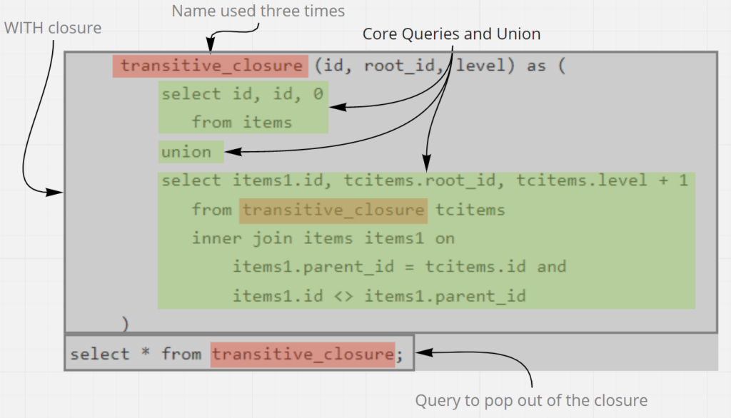
Focusing in on the CTE let’s analyse its parts

  • A language closure (WITH). (Note this is a different concept than transitive closure.)
  • A name
  • Core Queries and Union
  • Final query.

As it turns out 3/4 of this structure may be dropped without loss.

SQL – SELECT … UNION SELECT … FROM UNION

We propose simplifying SQL by dropping the name, the closure and the final query and simplifying the composable recursive relational query down to:

select id, id root_id, 0 level 
    from items
union
select items1.id, tcitems.root_id, tcitems.level + 1
    from union tcitems
        inner join items items1 on items1.parent_id = tcitems.id 
        and items1.id <> items1.parent_id

This form:

SELECT ... UNION SELECT ... FROM UNION

SELECTs the fixed-point result of the UNION without the overhead of a name (repeated three times), the closure and the final query.

This demonstrates that CTE machinery is not required to express recursive fixed point relational queries.

The simplified recursive relational query is orthogonal to all constructs in SQL and is composable:

  • if it is desired to hide some of the columns included in the recursive query, then the simplified recursive query can be wrapped in an outer SELECT, and
  • if the simplified recursive query needs to be consumed by more than one query then it can be
    • wrapped in a CTE, or
    • wrapped in a VIEW.

Multi-UNION Queries

There do need to be disambiguation rules if there are multiple UNIONs in scope. However, this is true whatever the linguistic form. See for example the multi-UNION rules for Sqlite. All non-recursive UNION sub-queries are constrained to be first, and all recursive sub-queries follow. And each recursive sub-query is presented with all generated rows from every other subquery in the UNION.

Composability

To be fair, the CTE variant of recursive queries is composable and SELECT FROM (WITH RECURSIVE …. SELECT …) works (at least in Sqlite). However, the ergonomics are poor, requiring the developer to build a mental model that includes a linguistic closure, a temporary local name, and a SELECT to pop back out of the closure. Here is the equivalent composable CTE-based query (Sqlite) with the required extra machinery in bold.

select * from (
with _unionfixedpoint (id, root_id, level) as (
select id, id root_id, 0 level from items union select items1.id, tcitems.root_id, tcitems.level + 1 from _unionfixedpoint tcitems inner join items items1 on items1.parent_id = tcitems.id and items1.id <> items1.parent_id)
select * from _unionfixedpoint
);

Application for other languages

The simplification of the recursive relational query to its essence is designed to improve developer experience and also points to a pattern for incorporating recursive queries into another language Morel.

Morel – from … union … from … in query

Having separated the idea of a recursive relational query from the CTE machinery, it becomes straight forward to propose the analog for a future release of Morel:

(from item in items 
    yield {id = item.id, root_id=item.id, level=0})
union
(from tcitem in query,
    item1 in items
    where item1.parent_id = tcitem.id and item1.id != item1.parent_id
    yield {id = item1.id, root_id=tcitem.root_id, level=tcitem.level+1});

The form

in query

is proposed for Morel, because ‘in union’ is too specific. Morel’s roadmap includes consideration for other UNION-like operators including unnamed lambdas.

Aligning Real Estate Agent’s interests with those of the Vendor

The interests of property sellers (vendors) and the interests of their real estate agent can be better aligned. Firstly, this article shows how the “x% on sale price” commission model fails to reward agents for the effort required to find the highest paying buyer for a property and leads to agents overquoting the expected property price. And secondly this article, proposes a “Shared Outcomes Commission Rates” model that more closely aligns the interests of the agent, with those of the seller. You can try it out here.

x% on sale price commission model

The “x% on sale price” commission model rewards the agent with a percentage (for example 2.5%) of the sale price. If the property sells for $1M then the agent’s commission would be $25K.

This commission model doesn’t reward the effort required by an agent to find the buyer who will pay a higher price. Let’s say that to sell the property at the expected sale price of $1M it takes an effort. If the agent doubled their efforts (or worked twice as smartly) to find the best buyer, would we expect the sale price to double to $2M? Hardly! It might sell for $1.1M or $1.2M or more depending on the context. This means that the doubly hard working (or doubly smart working) agent is at best rewarded +10% or +20% in their commission from the sale. The effect of this commission structure is that the smart agent will do just enough to attract a reasonable purchase offer and move on to the next sale.

As well, the “x% on sale price” commission model leads to conditions where an agent can raise the vendor’s expectations of the achievable sale price for the purpose of securing the agency for the property. The vendor’s interests are in a higher sale price, and the “x% on sale price” commission model means that even if the agent is only able to deliver an ‘average’ rather than ‘excellent’ result, the agent’s commission may only decrease by a small margin.

Let’s explore the root of these issues.

The bulk of the reward is for hardly any effort

If the vendor was willing to accept 80% of their property’s value it will sell itself. Why is it a promising idea to base 80% of an agent’s expected reward on just the fact that the vendor signed up with this particular agent?

Before moving on to more detail, please be assured that I am not trying to argue that agent commissions are too high or too low. Just that agent effort is not being rewarded where it delivers value.

My main question is this “Can we structure commissions so that the extra agency effort required to achieve a 110% or 120% sale price are rewarded properly?”

Rewarding agent effort

A “sale within some time period for 80% sale price” can be achieved with minimal agency effort. Let’s imagine a commission structure that promised the agent a minimal reward for that outcome and instead shifts commission to reward the effort required for more than the minimal outcome.

Moving the sale price from 80% of expectation to 100% will be possible at some level of agency effort and for double the agency effort the sale price might be moved from 100% of expectation to 110% or 120%. It would be good if that extra agency effort were rewarded by a commensurate increase in commission.

Another desirable feature of such a pricing structure is that the agent will be reluctant to recommend that a property be sold below the expected price, because their commission would fall away rapidly. A 10% fall in price might mean that the vendor gets 90% of the value of the property but the agent only gets 50% of their expected commission.

Agent motivation to fairly represent the expected sale price

Under the “x% on sale price” commission model, an agent can use a 10-20% over-estimation of the sale price to secure a listing and thereby gain the uncontested 80% of the commission.

A vendor is likely to prefer a commission structure would act in such a way that an agent’s failure to achieve the estimated sale price would result in a significant reduction in commission. Under this situation, an agent’s desire to overquote to secure the business would be balanced by their assessment of their ability to deliver the estimated sale price.

Tiered Commission Rate approach

One existing approach to addressing these concerns is tiered commission rates. For example, Open Agent Australia’s 2018 article on “Why we like tiered commission rates.” clearly outlines the challenge and proposes a tiered approach to commissions that addresses them.

However, in practice, it is not easy to set up tiered commission rates. Setting up tiering requires making dozens of inter-locking choices:

  1. how many tiers should we use,
  2. at what point should our tiers start and finish,
  3. how much should we increase the commission at each tier?
  4. And finally once it is setup, how do we communicate the impact on the agent and vendor of these decisions.

The Shared Outcome Commission Rates approach below vastly simplifies this down to just four decisions. Let’s see how it works.

Shared Outcome Commission Rates

The “Shared Outcome Commission Rates” structure described below is an original contribution by the author. If anyone is aware of this proposal being previously described, I would be happy to add citations to the earlier authors’ works.

A Shared Outcome Commission Rates structure aligns the interests of the vendor and the agent. Here is how is an illustration of how it works. We make four decisions to create the Shared Outcomes Commission Rates Structure

  1. Base Sale Price. Property is estimated to sell for (example) $1M based information available in the marketplace.
  2. Commission payable on Base Sale Price. (example) 2.2%
  3. Estimated Sale Price if agent doubles effort (or works doubly smart). (example) $1.1M
  4. Maximum incremental commission on additional sale price. Never more that (example) 25c in the dollar of increased sale price.

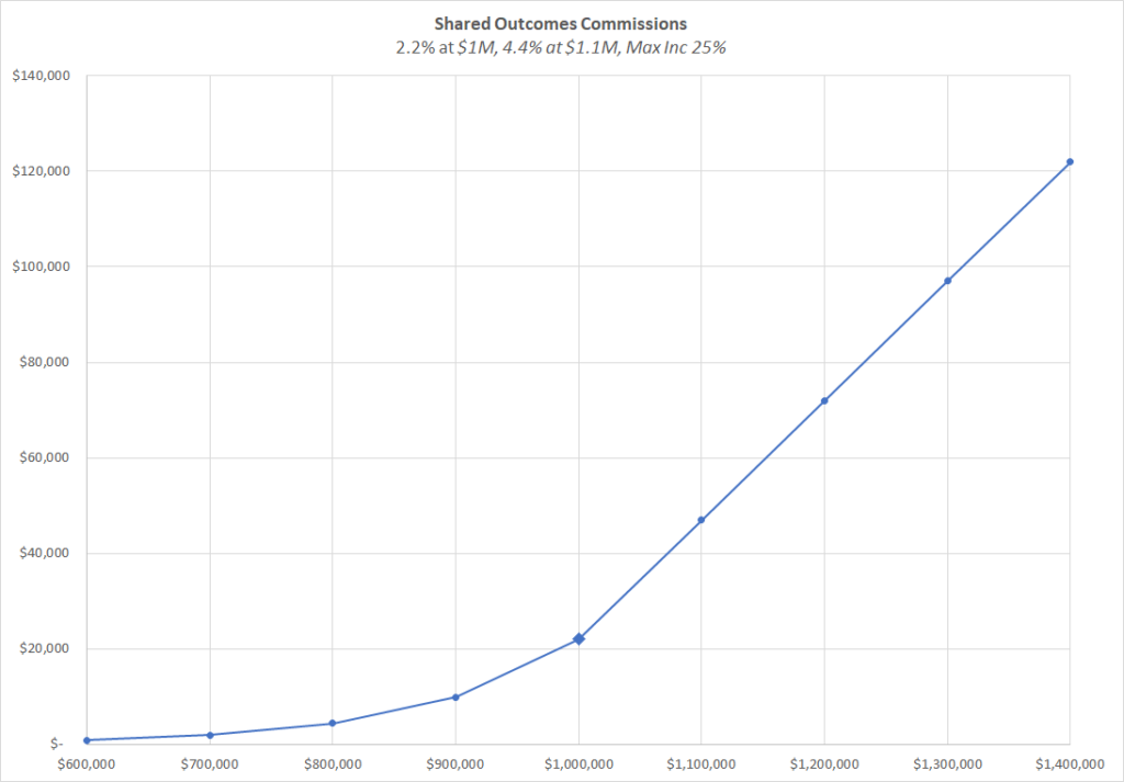
Using these four decisions Chart 1 shows a commission model that shares the outcomes between the vendor and agent in proportion to the outcomes/ effort.

Chart 1. Shared Outcome Commission Rates
2.2% at $1M, 4.4% at $1.1M, Max Inc 25%

As you can see from Chart 1. above, a sale price 10% higher will attract double the commission and a sale price 10% worse, will attract a 50% commission of just 1.1%

The straight-line part on the right-hand side of the commission curve is caused by the decision to never allocate more than 25c in any dollar towards commissions.

Try it yourself

A Shared Outcomes Commission Rates calculator is here: https://davidpratten.com/sharedoutcomescommissionrates

Adjusting for market conditions

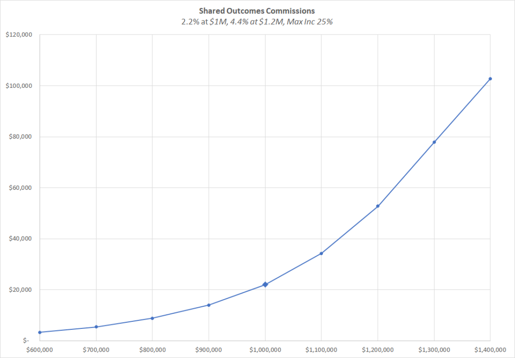
By way of comparison, if the market uncertainties were higher and a ten percent improvement could just occur by chance but a 20% improvement on the sale price is expected to require double the agent effort then the following Shared Outcomes Commission Rates structure might be more suitable.

Chart 2. Shared Outcome Commission Rates
2.2% at $1M, 4.4% at $1.2M, Max Inc 25%

Under this scenario, while the agent has a slower increase in commissions on the upside, it now takes a full 20% fall in sale price to halve the commission payable to the agent.

Impact of Shared Outcome Commission Rates

The author believes that the proposed “Shared Outcomes Commission Rates”, will positively align the interests of vendors and real estate agents.

  • Agents are rewarded in proportion to their efforts when delivering superior outcomes. And not rewarded for over-estimating the sale price.
  • And vendors are no longer paying 80% of the commission just because they signed up with an agent.

Win – Win.

Try it out … https://davidpratten.com/sharedoutcomescommissionrates

GA 382 | Simplifying Value Stream Mapping with Steve Pereira

This week’s guest is Steve Pereira. Steve and Ron discussed Steve’s minimalist approach to value stream mapping, and how it differs from other approaches. Steve doesn’t have a traditional lean background, but his perspective is refreshing and unique.

Source: GA 382 | Simplifying Value Stream Mapping with Steve Pereira

Feds list the top 30 most exploited vulnerabilities. Many are years old

Enlarge (credit: Getty Images ) Government officials in the US, UK, and Australia are urging public- and private-sector organizations to secure their networks by ensuring firewalls, VPNs, and other network-perimeter devices are patched against the most widespread exploits.

Source: Feds list the top 30 most exploited vulnerabilities. Many are years old

Kids set free to roam on their own feel more confident navigating in adulthood

Boys are often allowed to stray farther from home without adult supervision than girls are. Imgorthand/E+ Collection via Getty Images The distance from home that kids are allowed to roam and play has shrunk significantly over the last 50 years.

Source: Kids set free to roam on their own feel more confident navigating in adulthood

Earth’s inner core is growing more on one side than the other – here’s why the planet isn’t tipping

Argonne National Laboratory/flickr , CC BY-NC-SA More than 5,000 kilometres beneath us, Earth’s solid metal inner core wasn’t discovered until 1936 . Almost a century later, we’re still struggling to answer basic questions about when and how it first formed.

Source: Earth’s inner core is growing more on one side than the other – here’s why the planet isn’t tipping

Here is a brief history of toilets

Who gives a crap about the history of toilets? Francis de los Reyes does. He’s a professor of civil engineering at North Carolina State University whose research focuses on “wastewater treatment plant design, environmental biotechnology and microbiology, fundamentals of environmental engineering, and water and sanitation for developing countries.” — Read the rest

Source: Here is a brief history of toilets

Weeknotes: datasette-remote-metadata, sqlite-transform –multi

I mentioned Project Pelican (still a codename until the end of the embargo) last week . This week it inspired a new plugin, datasette-remote-metadata . I also published an article describing the Baked Data architectural patttern and shared the video and transcript of a talk I gave at PyGotham last year. datasette-remote-metadata Datasette’s metadata system is one of the key ways of customizing a Datasette instance: it lets you add extra information about the tables hosted by the instance, lets you configure canned queries and also (due to some scope creep that I’d love to clean up ) lets you configure options for various Datasette plugins.

Source: Weeknotes: datasette-remote-metadata, sqlite-transform –multi

Compendium of Blog Posts for Managing in the Presence of Risk

Risk Management is How Adults Manage Projects – Tim Lister What is Risk? What is Risk Management? Six Common Pitfalls of Risk Management Retrospective Coherence – What Does That Mean ? Risk Management is Project Management for Adults – Tim Lister Risk Management is How Adults Manage Projects Risk Management is How Adults Manage Projects (Part 2) Risk Management of How Adult Manage Projects (12.0 of Workshop) Risk Management is How Adults Manage Projects: Agile is Not Risk Management (Alone) Risk Management is How Adults Manage Projects (Susanne Mades talk) Risk Management is How Adults Manage Project (Critical Uncertainties) Risk Management is Project Management for Adults (Tim Lister’s talk) Acting Like an Adult in the Presence of Uncertainty A Quick Summary of Risk Management The Profession of Risk Management and its Value to Project Success Beyond the Risk Register Six Steps of Risk Management Risk, Their Sources, and Handling Strategies Risk Management in Five Easy Pieces, with Apologies to Jack Both Aleatory and Epistemic Uncertainty Creat Risk Epistemic and Aleatory Uncertainty Creates Risk to Project Success Aleatory Uncertainty Creates Irreducible Risk Epistemic Uncertainty Creates Reducible Risk How Do Projects Fail?

Source: Compendium of Blog Posts for Managing in the Presence of Risk

✚ Visualization Tools and Learning Resources, July 2021 Roundup

Welcome to issue #150 of The Process , the newsletter for FlowingData members about how the charts get made. I’m Nathan Yau, and every month I collect tools and resources that help you visualize data better. This is the good stuff for July.

Source: ✚ Visualization Tools and Learning Resources, July 2021 Roundup

Table Valued Constrained Functions (TVCF) – Constraint Programming and SQL

I propose seamless integration of solvers into SQL via Table Valued Constrained Functions (TVCF). By "seamless", I mean that the SQL programmer would have to ask the query planner if a constraint solver was invoked to complete the query.

A few years ago, I sketched the design of an ideal logic and constraint-based language "Parasat". In this article I describe a SQL language extension with similar goals which is also inspired by Picat.

Motivating Example

At university I was surprised, and disappointed, by the distance between the predicates of mathematical logic and those of Prolog. For example the Prolog interpreter was unable to give the answers

X=-4, Y= -3 and X=3 and Y=4 

to the simultaneous equations x+1-y = 0 and x^2+y^2-25 = 0 expressed in Prolog as this predicate:

simultaneous(X,Y) :- plus(X, 1, Y),times(X,X,XSquared),times(Y,Y,YSquared),
    plus(XSquared,YSquared, XSquaredPlusYSquared),equals(XSquaredPlusYSquared,25)

Here is another way forward by extending SQL’s Table Valued Functions (TVF) to include constraints passed into the function by the query planner.

Solving this simultaneous equation with SQL-92

This particular simultaneous equation can be solved using an ordinary garden variety SQL-92 SELECT query. Given two relations, one each for the simultaneous equations:

CREATE TABLE XPlusZEqualsY (X,Z,Y);
CREATE TABLE XSquaredPlusYSquaredEqualsZ(X,Y,Z);

populated with select rows as follows:

XPlusZEqualsY

X Z Y
-5 1 -4
-4 1 -3
-3 2 -1
-3 1 -2
2 1 3
3 1 4
4 3 7

XSquaredPlusYSquaredEqualsZ

X Y Z
-4 -3 25
-1 -1 1
0 0 0
3 4 25

The following SQL-92 SELECT query will solve the simultaneous equation:

SELECT
  r1.X,
  r1.Y
FROM
  XPlusZEqualsY r1
  INNER JOIN XSquaredPlusYSquaredEqualsZ r2 ON r1.X = r2.X AND r1.Y = r2.Y
WHERE r1.Z = 1 and r2.Z = 25;

However, this is not a useful technique. This SELECT query only works when, out of the infinite rows that could be in the relations, the specific rows that make the simultaneous equation true happen to be pre-loaded.

Can Table Valued Functions (TVF) be used to provide a generic solution?

No, is the short answer. What are TVFs and why can’t they provide a solution?

Table Valued Functions (TVF) are defined in the SQL standard and implemented in widely-used databases.

a table function returns a (relational) table comprising zero or more rows, each row with one or more columns. See wikipedia User Defined Functions

TVFs are implemented in a variety of databases for example: SQLite, PostgreSQL, and MS SQL.

TVFs can’t provide a general solution the simultaneous equation problem. The example above will illustrate this. If we replace the tables above with TVFs and pass the two TVFs some parameters:

Q: What parameters(?) would we pass them to ensure that the TVFs generated the correct rows to be selected against?

SELECT
  r1.X,
  r1.Y
FROM
  XPlusZEqualsY(?) r1
  INNER JOIN XSquaredPlusYSquaredEqualsZ(?) r2 ON r1.X = r2.X AND r1.Y = r2.Y
WHERE r1.Z = 5 and r2.Z = 25;

A: There aren’t any (non-magical) parameters that can achieve this.

Table Valued Constrained Functions (TVCF)

As defined in this article, TVCFs are like TVFs in that they are:

  • Functions
  • that return 0 or more rows of 1 or more columns

In addition, however, TVCFs:

  • have a fixed and typed column-set, like an ordinary table or view
  • are read-only (no UPDATE or DELETE FROM),
  • may delegate back to the query planner the task of generating the next value by invoking a solver
  • are possibly non-deterministic
  • appear in SQL code as just their name like a table or a view (i.e. without parameters)
  • are lazily evaluated
  • are defined in a language which can be compiled into a form usable by solvers. We know this is feasible because the language Picat has this property.
  • parameters to the TVCF are provided by context e.g. constraints provided by ON and WHERE clauses

When a TVCF is referenced in a query:

  • if the contextually provided constraints provide all the information required to generate the next row the function returns the next row to the query engine.
  • otherwise the TVCF invariant is compiled by the query planner and with the known constraints is passed as input into a solver. The query planner seamlessly consumes the solver output and continues with the query.

What is a solver?

A solver accepts constraints specified in some language and provides solutions using one or more techniques. A good introduction to solvers may be found:

TVCFs Example

Here is the XPlusZEqualsY table from our example coded as a TVCF using a pythonic idiom:

CREATE FUNCTION XPlusZEqualsY 
    (X float|[constraint,..], 
    Z float|[constraint,..], 
    Y float|[constraint,..])
RETURNS TABLE
AS
INVARIANT: X+Z-Y=0
IF X, Z, and Y are float:
    /* All parameters are provided */
    IF INVARIANT(X,Z,Y):
        RETURN (X,Z,Y)
    ELSE:
        RETURN(EMPTY_ROW())
/* Two out of three parameters */
IF X and Z are float:
    RETURN (X, Z, X+Z)
ELIF X and Y are float:
    RETURN (X, Y-X, Y)
ELIF Z and Y are float:
    RETURN (Z-Y, Y, Z)
ELSE:
    /* less than two parameters */
    DELEGATE INVARIANT,X,Z,Y
;

This function has:

  • named input parameters of X, Z, and Y which are either floats or a list of constraints on the value of the parameter.
  • named result columns of X, Z and Y which are always floats.

The INVARIANT line captures the intent of the relation in a form:

  • usable as a true/false predicate, and
  • compilable to a form usable by a solver.

Let’s walk through the flow of the function

The behaviour of the function (copied at right) depends on what is provided by the query planner based on the context.

All parameters are provided. As would be the case in this example:

SELECT 1 FROM XPlusZEqualsY 
    WHERE X=1 AND Z=2 AND Z=3;

In this case, the provided row is returned if the invariant is true otherwise there is no matching value in the relation and the empty row is returned.

Two out of three parameters are provided. As would be the case in this example:

SELECT Z FROM XPlusZEqualsY 
    WHERE X=1 AND Y=2;

In this case the missing value is computed and the three values are returned as a row.

One or fewer parameters are provided. As in our example above (copied here for convenience):

SELECT
  r1.X,
  r1.Y
FROM
      XPlusZEqualsY r1
  INNER JOIN 
      XSquaredPlusYSquaredEqualsZ r2 
  ON r1.X = r2.X AND r1.Y = r2.Y
WHERE r1.Z = 1 and r2.Z = 25;

Here we have Z constrained to be 1 but X and Y are merely constrained not specified. In this case, the invariant with the parameters are delegated back to the query planner to compile and submit to a heuristically chosen solver.

CREATE FUNCTION XPlusZEqualsY 
    (X float|[constraint,..], 
    Z float|[constraint,..], 
    Y float|[constraint,..])
RETURNS TABLE
AS
INVARIANT: X+Z-Y=0
IF X, Z, and Y are float:
    /* All parameters are provided */
    IF INVARIANT(X,Z,Y):
        RETURN (X,Z,Y)
    ELSE:
        RETURN(EMPTY_ROW())
/* Two out of three parameters */
IF X and Z are float:
    RETURN (X, Z, X+Z)
ELIF X and Y are float:
    RETURN (X, Y-X, Y)
ELIF Z and Y are float:
    RETURN (Z-Y, Y, Z)
ELSE:
    /* less than two parameters */
    DELEGATE INVARIANT,X,Z,Y
;

Summary Pitch

SQL query writers are specifying constraints all the time, by using Table Valued Constrained Functions (TVCF) they gain access to the power of solvers with zero learning friction. Those responsible for writing SQL query planners are already using solver toolkits to solve other database challenges and are well placed to incorporate them into the heart of the relational model.

I just found three bugs in SQLite!

SQLite is the most widely used and arguably the most rigorously tested database in the world.

Today, the developers confirmed that valid queries that I created for the Rosella Model project exposed not one, not two, but three bugs hiding in the code.

I really can’t remember the last time a single query found 2 bugs, let alone 3. Quote source

Reflecting on the spirit of my work, one of the developers said

For years, I’ve been giving talks that encourage developers to embrace the power of the SQL query language – to move beyond simple SELECT and INSERT statements mixed with a pile of procedural code and instead write complex queries that give the answer directly. I often use some of the queries generated by Fossil as examples, pointing out how a few lines (or a few dozen lines) of SQL can replace thousands and thousands of lines of procedural code. Doing so reduces the number of bugs (which are roughly proportional to the number of lines of code) and also often result in faster solutions as well. But you, sir, have taken this idea to a whole new level. Quote source

I’m happy to claim bragging rights!